
Using Machine Learning to Predict Top Tracks
1. Background
I will be using the same data pulled from Part 1 for this analysis. See Part 1 for details on how this dataset was created. After combining data from Billboard, Spotify, and Genius, I chose to focus on two questions:
- How has rap changed over the years? Can I represent this visually?
- Is it possible to accurately predict which tracks will break into the top 5 spots on Billboard? Do top 5 rap songs across all years share any similarities?
This notebook will focus on pulling, combining, and cleaning data in addition to developing insights for the second question above.
The analysis resulted in the following conclusions:
- Random forest was the best model but still had trouble predicting a track correctly as “Top 5”. This suggests that top 5 tracks are very diverse on an audio feature basis.
- Features derived from the actual lyrics will likely be needed to improve model performance (common words, bigrams, and trigrams).
2. Data Preparation
import pandas as pd
import numpy as np
import matplotlib.pyplot as plt
import seaborn as sns
sns.set()

%matplotlib inline

complete_df_3 = pd.read_pickle("complete_3.pkl")
complete_df_3["week"] = pd.to_datetime(complete_df_3["week"])data_df = complete_df_3.groupby(by=["artist","title"], as_index=False).apply(lambda x : x[x["current_rank"]==(x["current_rank"].min())])
data_df = data_df.sort_values(by=["week","current_rank"],ascending=[False,True])#Drop duplicate track rows, keeping only the first occurrence of when the track reached its top spot on the charts
data_df = data_df.drop_duplicates(subset=["artist","title"],keep="last").reset_index(drop=True)#Target column: 1 if it peaked in the top 5 else 0
data_df["top_5"] = data_df["peak_pos"].apply(lambda x : 1 if x<=5 else 0)#Below, I noticed that I had imbalanced classes which would need to be addressed
data_df["top_5"].value_counts()0 2289
1 7963. Predictive Modeling
3.1. Data Split, Scaling, and SMOTE-NC
Next, it was time to build some machine learning models. I used the macro-F1 score to compare models. First, I filtered the columns I wanted to use as features into variable X and set the target variable to y. I used a stratified split into a train and test set. Then I split the train set into 5 stratified folds for cross-validation.
from sklearn.linear_model import LogisticRegression
from sklearn.model_selection import StratifiedShuffleSplit, train_test_split
X = data_df[["explicit", "danceability","energy","loudness","speechiness","acousticness","valence",
"mean_sentiment","std_sentiment","duration_sec","words_per_second","unique_word_proportion"]]
X["explicit"] = X["explicit"].astype("category")
y = data_df["top_5"]from sklearn.model_selection import train_test_split
X_train, X_test, y_train, y_test = train_test_split(X, y, test_size=0.2, random_state=5, stratify=y)
from sklearn.model_selection import StratifiedKFold
kf = StratifiedKFold(n_splits=5, shuffle=True, random_state=20)from sklearn.preprocessing import StandardScaler
#We will scale all non-binary columns
scaler = StandardScaler()
X_train_scaled = X_train
X_test_scaled = X_test
X_train_scaled.loc[:,X_train_scaled.columns!="explicit"] = scaler.fit_transform(X_train_scaled.loc[:,X_train_scaled.columns!="explicit"])
col_mean = scaler.mean_
col_std = (scaler.var_)**.5
X_test_scaled.loc[:,X_train_scaled.columns!="explicit"] = (X_test.loc[:,X_train_scaled.columns!="explicit"]-col_mean)/col_stdNext, I used the synthetic minority oversampling technique (SMOTE) which required installation of the following module:
pip install imbalanced-learnThis technique generates additional samples from the non-majority classes so that the resulting data set has an equal representation for all classes. These additional samples are not simply copies of existing rows. Instead, the algorithm utilizes a nearest neighbors approach to synthesize new data points.
A major challenge that arose was how to incorporate SMOTE into grid search and cross-fold validation. The synthetically generated training samples depend on the original training set. As a result, my decision to use 5 stratified folds essentially meant that 5 different SMOTE generated training sets would be needed. The below code solves this issue by generating a SMOTE training set for each of the 5 folds and saving the corresponding SMOTE training vs cross-validation indices into the cv_indices list.
from imblearn.over_sampling import SMOTENC

sm = SMOTENC(categorical_features=[0], random_state= 17)

X_train_custom = X_train_scaled.reset_index(drop=True)
y_train_custom = y_train.reset_index(drop=True)
num_rows_original = X_train_custom.shape[0]

smote_indices = []
cv_indices = []

fold_num=0
for train_index, cv_index in kf.split(X_train_custom,y_train_custom):
    num_rows_fold_original = len(train_index)
    X_train_smote_fold, y_train_smote_fold = sm.fit_sample(X_train_custom.iloc[train_index],
                                                           y_train_custom.iloc[train_index])
    X_train_smote_fold = X_train_smote_fold.iloc[num_rows_fold_original:]
    y_train_smote_fold = y_train_smote_fold.iloc[num_rows_fold_original:]
    X_train_custom = pd.concat([X_train_custom,X_train_smote_fold],ignore_index=True)
    y_train_custom = pd.concat([y_train_custom,y_train_smote_fold],ignore_index=True)
    if fold_num==0:
    smote_indices.append([*range(num_rows_original,num_rows_original+X_train_smote_fold.shape[0])])
    else:
        last_row = smote_indices[-1][-1]
        smote_indices.append([*range(last_row+1,last_row+1+X_train_smote_fold.shape[0])])

    train_index_fold = np.append(train_index,smote_indices[fold_num])
    cv_index_fold = cv_index
    cv_indices.append((train_index_fold,cv_index_fold))

    fold_num+=1
Finally, I ran SMOTE on the entire training set (without leaving any data out for cross-validation).
X_train_smote, y_train_smote = sm.fit_sample(X_train_scaled, y_train)
y_train_smote.value_counts()
kf = StratifiedKFold(n_splits=5, shuffle=True, random_state=20)
1 1831
0 18313.2. Logistic Regression
X_train_smote, y_train_smote = sm.fit_sample(X_train_scaled, y_train)
y_train_smote.value_counts()from sklearn.model_selection import GridSearchCV
from sklearn.linear_model import LogisticRegression

log_params = {"penalty":["l1","l2"],
              "C":[.0001,.001,.01,.1,1,10,100,1000,3333,10000,33333,100000],
              "random_state":[20],
              "solver":["liblinear"],
              "max_iter":[1000]}
log = LogisticRegression()
log_grid = GridSearchCV(estimator=log,
                        param_grid=log_params,
                        scoring="f1_macro",
                        cv=cv_indices)
log_grid.fit(X_train_custom, y_train_custom)log_grid.best_params_{'C': 10,
'max_iter': 1000,
'penalty': 'l1',
'random_state': 20,
'solver': 'liblinear'}log_grid.best_score_0.55613626582679243.3. K-Nearest Neighbors
While the above logistic regression was quite promising, I wanted to see if other ML models would result in better performance. I next built a KNN model. Given that I did not have that many features, I used all of them for this analysis.
from sklearn.neighbors import KNeighborsClassifier
knn_params = {"n_neighbors" : [2,4,8,16,32,64,128,256,512,1024],
              "weights" : ["uniform", "distance"],
              "p" : [1,2]}
knn = KNeighborsClassifier()
knn_grid = GridSearchCV(estimator=knn,
                        param_grid=knn_params,
                        scoring="f1_macro",
                        cv=cv_indices)
knn_grid.fit(X_train_custom[log_features], y_train_custom)knn_grid.best_params_{'n_neighbors': 2, 'p': 2, 'weights': 'uniform'}
knn_grid.best_score_0.530958495897352
3.4. Support Vector Machine
from sklearn.svm import SVC
svm_params = {"C":[.0001,.001,.01,.1,1,10,100,1000],
              "kernel":["poly","rbf"],
              "degree":[2,3]}
svm = SVC()
svm_grid = GridSearchCV(estimator=svm,
                        param_grid=svm_params,
                        scoring="f1_macro",
                        cv=cv_indices,
                        verbose=3)
svm_grid.fit(X_train_custom, y_train_custom)svm_grid.best_params_{'C': 0.1, 'degree': 2, 'kernel': 'rbf'}
svm_grid.best_score_0.5590538164185677
3.5. Random Forest
from sklearn.ensemble import RandomForestClassifier
rf_params = {"n_estimators" : [100],
             "max_depth" : [2,4,8,16,32,64,128,None],
             "max_features" : ["sqrt", "log2", .1, .25, .5, 5, 10, 25],
             "min_samples_leaf" : [1,3,5],
             "random_state" : [10]}
rf = RandomForestClassifier()
rf_grid = GridSearchCV(estimator=rf,
                       param_grid=rf_params,
                       scoring="f1_macro",
                       cv=cv_indices,
                       verbose=3)
rf_grid.fit(X_train_custom, y_train_custom)rf_grid.best_params_{'max_depth': 16,
'max_features': 0.1,
'min_samples_leaf': 5,
'n_estimators': 100,
'random_state': 10}rf_grid.best_score_0.5615439525222539
3.6. Model Selection and Interpretation
The results of the above models are summarized in the table below (ordered from best to worst performance):
models = ["Logistic Regression",
          "K-Nearest Neighbors",
          "Support Vector Machine",
          "Random Forest"]

optimized_parameters = [log_grid.best_params_,
                        knn_grid.best_params_,
                        svm_grid.best_params_,
                        rf_grid.best_params_]

F1 = [log_grid.best_score_,
      knn_grid.best_score_,
      svm_grid.best_score_,
      rf_grid.best_score_]

model_df = pd.DataFrame({"model" : models,
                         "optimized_parameters" : optimized_parameters,
                         "macro-F1" : F1})

with pd.option_context('display.max_colwidth', 150):
    display(model_df.sort_values(by="macro-F1",ascending=False))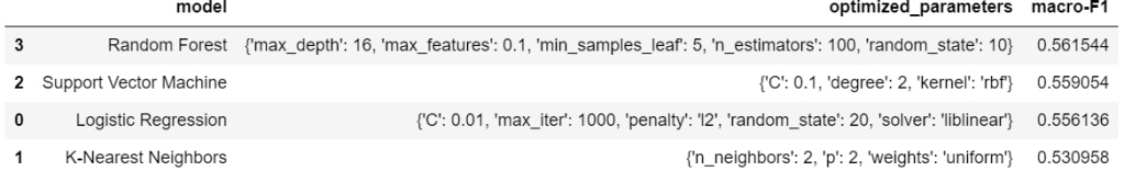
The random forest model performed the best, although the macro-F1 score was quite similar across models. I ran the random forest model with the optimized parameters on the test set for a final assessment of macro-F1.
#Fit model to entire SMOTE training set
model_best = RandomForestClassifier(max_depth=16,max_features=.1,min_samples_leaf=5,n_estimators=100,random_state=10)
model_best.fit(X_train_smote,y_train_smote)

#Predict test values
y_pred = model_best.predict(X_test)

#Calculate weighted-F1
from sklearn.metrics import f1_score
f1_score(y_test,y_pred,average="macro")
0.5634600022823233
Next, I built a confusion matrix. The model clearly had trouble correctly predicting “Top 5”.
from sklearn.metrics import confusion_matrix
sns.set(font_scale=1.6)
cm = confusion_matrix(y_test, y_pred)
fig, ax = plt.subplots(figsize=(16,12))
sns.heatmap(cm, annot=True, ax = ax, fmt="d")
ax.set_xlabel('Predicted')
ax.set_ylabel('True')
ax.set_title('Confusion Matrix')
ax.xaxis.set_ticklabels(["Not Top 5", "Top 5"])
ax.yaxis.set_ticklabels(["Not Top 5", "Top 5"])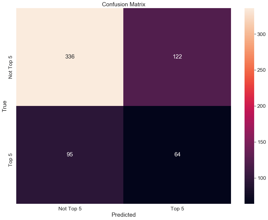
4. Conclusion/Further Steps
The chosen random forest model had trouble identifying Top 5 tracks. It is very possible that the features I chose are not adequate to make accurate predictions, as Top 5 tracks are very diverse.
As a first additional step, I would conduct error analysis by randomly choosing some misclassified tracks. If a pattern was evident as to why tracks were consistently misclassified, I could adjust the model/add more complicated features to improve it. Second, I would include additional features extracted from the actual lyrics of the tracks. Perhaps the presence of certain words, bigrams, or trigrams would aid in prediction. I also suspect that non-musical features, such as marketing budget, general popularity of the artist, etc. have a significant influence of which tracks break into the top spots.
